Raw Data Vault to Star Schema

Overview

In a prior blog, Data Vault Acceleration with Kyvos Smart OLAP™, I describe how the Data Vault Methodology 2.0 is an advancement over the traditional means for building data warehouses. In this blog, I focus on the Kimball Data Warehouse methodology, which is the E-T-L into a star/snowflake structured data warehouse.

However, I need to stress that a Data Vault is actually two parts in one – the Raw Data Vault and the Business Vault. The two parts cater to different needs relating to loading the data into the data warehouse and consuming the data in the data warehouse.

To explain this difference, let’s first consider that the means for populating a newer Data Vault versus an older star/snowflake data warehouse has a corresponding difference. I’m referring to the currently favored E-L-T as an advancement of the older E-T-L.

For the older E-T-L, data was (E)xtracted from source systems, all sorts of (T)ransformations (cleansing, mapping, etc.) were performed, and that metamorphosed data was (L)oaded into a star/snowflake schema enterprise data warehouse (EDW). The EDW presented to end-users is clean, trustworthy, and user-friendly, and at least reasonably performant.

The main problem was that before data landed into the EDW, all the transformations (the “T” in ETL or ELT) had to be worked out. That one little letter, “T”, represents a world of pain. For example, different domains need to hammer out the meaning of nouns such as “customer”, “sale”, or “profit”. Or how to convert from one unit to another. Or which system holds the “correct” version of what should be the same thing but isn’t. Such definitions and business rules, are surprisingly difficult to work through.

To rectify that bottleneck, the dual concepts of E-L-T and Data Lakes came along. Similar to E-T-L, data is first (E)xtracted data from source systems. But the dreaded T is postponed. Instead, (L)oading the data is loaded into a highly-scalable data lake with minimal or no transformations. This way, the many consumers have access to data much sooner and are free to apply (T)ransformations according to their own needs, in their own time, and can even change their minds.

The Data Vault is also an E-L-T methodology, even preceding the data lake. The raw data vault represents the E and L. The advantage of the raw Data Vault over the Data Lake is that the raw Data Vault imposes a level of schema structure that is versatile and easy to understand.

The versatility of the raw data vault structure enables near plug-a-play additions of new data sources. However, the versatility comes with a price. That price is a schema composed of many more tables than the older star/snowflake schema. That requires many more objects (DDL, ETL, etc.) to deploy, many more costly joins to process, and a less than ideal schema for human end-users to master.

The many objects to deploy isn’t usually that much of a problem since Data Vault implementations usually employ some sort of automation tool such as dbtVault, WhereScape, and Erwin. The benefit of strict adherence to the Data Vault methodology facilitates the feasibility for automation. However, the many joins can be a problem for query performance and the ability for human consumers to comprehend the raw data vault schema.

Therefore, a user-friendly layer must be lifted above the raw data vault. A layer better suited for direct human consumption. This is the Business Vault, an intermediary between the raw data vault and the consumer. Think of it as splitting the “T” in two parts. The first part can be thought of as the business vault meeting the consumer halfway with a human-friendly view. And the second part of the “T” being whatever business rules the user wishes to apply.

Data Vault to Star Schema

The subject of this blog isn’t directly about Kyvos Smart OLAP™ itself. This blog is about what happens just upstream from where I suggest employing Kyvos as a query performance acceleration layer for a data vault. There is seemingly a chasm between what is often thought of as the “data vault” and what Kyvos (or most other consumers of a data vault) would see.

That chasm, circled in red in Figure 1, is the jump to the lesser known “Business Vault”. In this case, the Business Vault includes star schemas that is presented as a schema Kyvos can readily consumable.

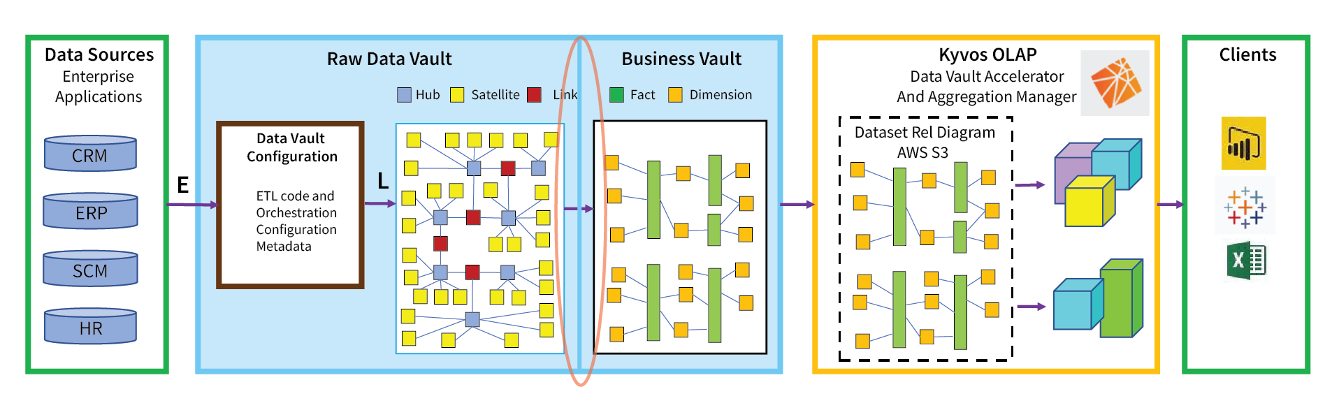
Figure 1 – This blog is about shedding some light on how we get from the raw data vault to the business vault.

This blog isn’t intended to comprehensively cover the subject of the business vault. Data Vault is a big and evolving subject. My intent for this blog is to provide insight into the general idea of getting from the raw data vault to the star/snowflake schemas that are most conducive towards analytics by users of Kyvos or other front-end means.

I must note as well that although I’m writing about star/snowflake schemas in the context of the business vault, the business vault consists of many other sorts of structures. For example, we will see a “Point-in-Time” (PIT) table. Additionally, the fact table (part of the star schema) is essentially another standard business vault structure called a “bridge table”. It’s that I focus on the star schema here because in the context of Kyvos, that is what is relevant.

In this blog my intent is to shed some light on the existence of the chasm between the raw data vault to the business vault. As depicted in Figures 2a and 2b, the schemas are very different, serving very different purposes.
Figure 2a depicts what is a very simple raw data vault schema for sales orders. Although the schema consists of seventeen tables, there are really only four dimensions: Customers, Store, Product, and Order.

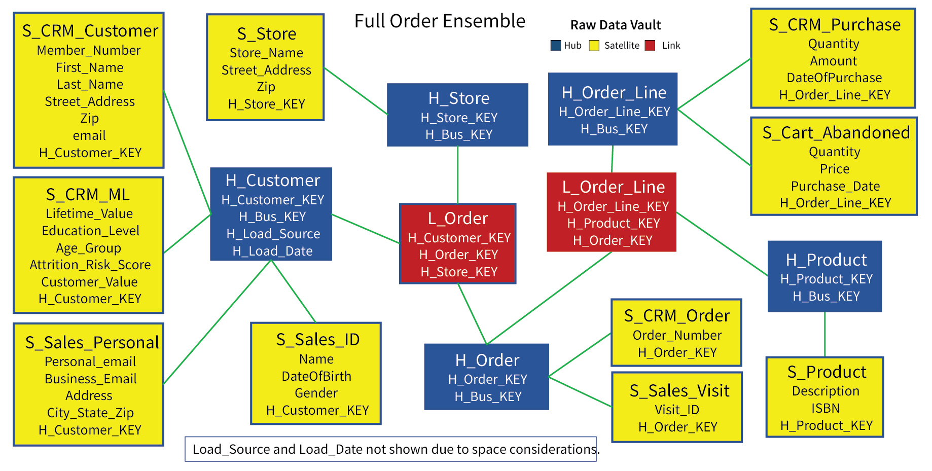
Figure 2a – A raw data vault ensemble of a sales orders.

Satellites (yellow) are generally the most plentiful type of table in the raw data vault. Each satellite is ideally a coherent column family partitioned from a larger set of hub entity attributes. The satellites in Figure 2a have been partitioned in the following ways:

1. There are two data two sources: The Customer Relationship Management (CRM) system and an online sales Web site (Sales). The latter includes information about orders that were cancelled and abandoned.
2. The customer entity (satellites of the H_Customer hub) is split into two column families each for the CRM and Sales systems.
   • a. For the CRM system, the S_CRM_Customer satellite holds typical customer information. The S_CRM_ML satellite was later added by data scientists.
   • b. The Customer Sales satellites are split along the lines of changing values. S_Sales_ID holds data that is very stable, very unlikely to change if at all. S_Sales_Personal holds customer information that tends to change on a slowly regular basis for most people.

Figure 2b depicts much a simpler, denormalized star schema lifted out of the raw data vault in Figure 2a.

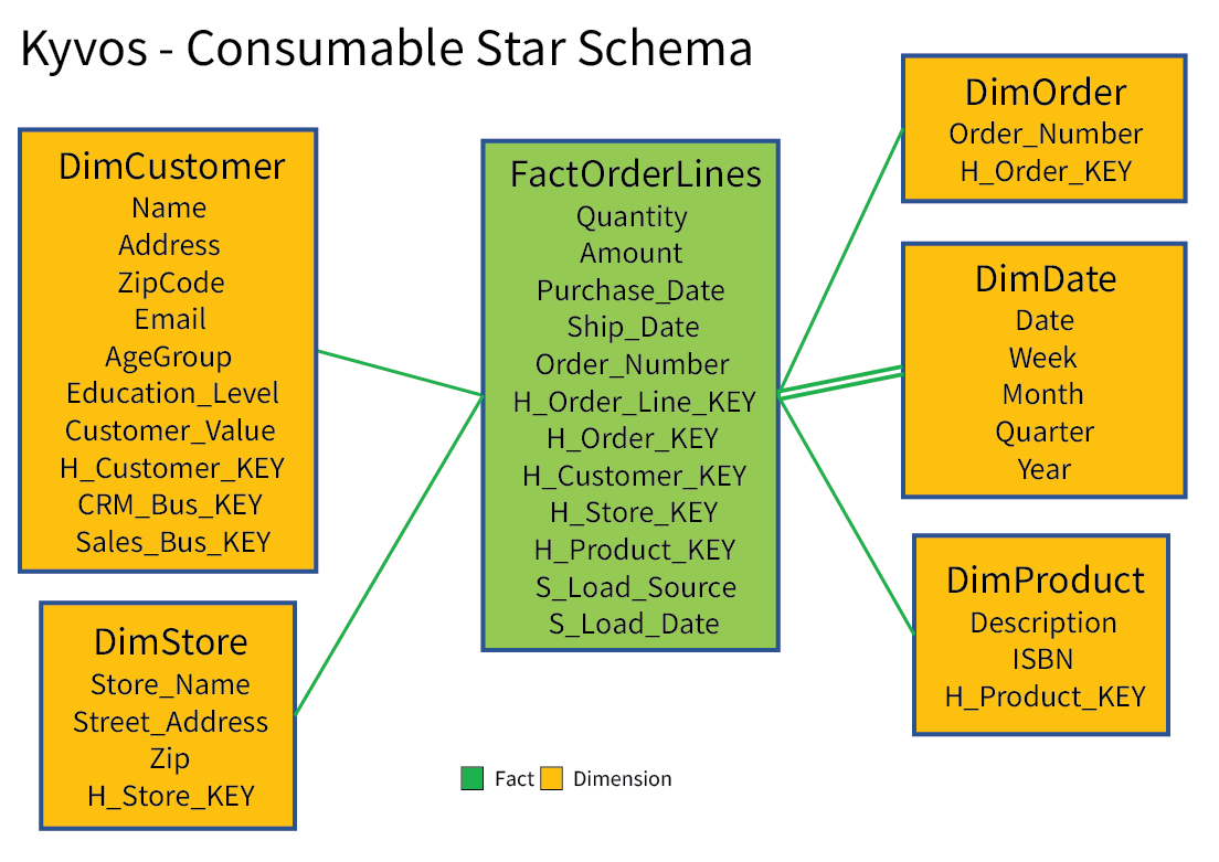
Figure 2b – An easily digestible Business Vault star schema pulled from the raw data vault ensemble.

The journey involved a few non-trivial intermediary steps dealing with issues of mapping customers from the two systems, application of business rules, and consolidating satellites into single dimensions. Being much easier to understand and highly performant, the star schema presents a preferable view for the human end users and a format conducive to Kyvos’ substantial performance acceleration capabilities.

It’s important to note that there can be more than one star schema plucked out of the raw data vault. In fact, there should be star schemas custom-fit to the various business requirements of analysts. The idea of E-L-T over the older E-T-L is that for E-L-T, the raw data can be transformed in multiple ways.

Additionally, the business vault is not limited to star schemas as the only human-friendly constructs. That includes variations of the star schema theme such as snowflake schema, multi fact table, or even a completely flattened table – which are very much consumable as the sources for Kyvos cubes.

The Raw Data Vault Metamorphosis

The road from raw data vault to star schema shouldn’t be that difficult if the patterns of the Data Vault Methodology are reliably followed. As a ballpark heuristic, I’d say the notion of Hubs take us about two thirds of the way towards your dimensions and Links get you at least halfway to fact tables.

Satellite columns supply the attributes of the dimensions. Satellites should be coherent column families related to some category or entity (Hub). By “coherent”, I mean that the columns in a satellite are somehow related. For example, in terms of semantics, or what is normally read together or written together.

Figure 3 depicts an abridged, combined version of Figures 2a and 2b above. By “abridged”, I mean some tables and columns are left out for the sake of fitting everything into a readable picture.

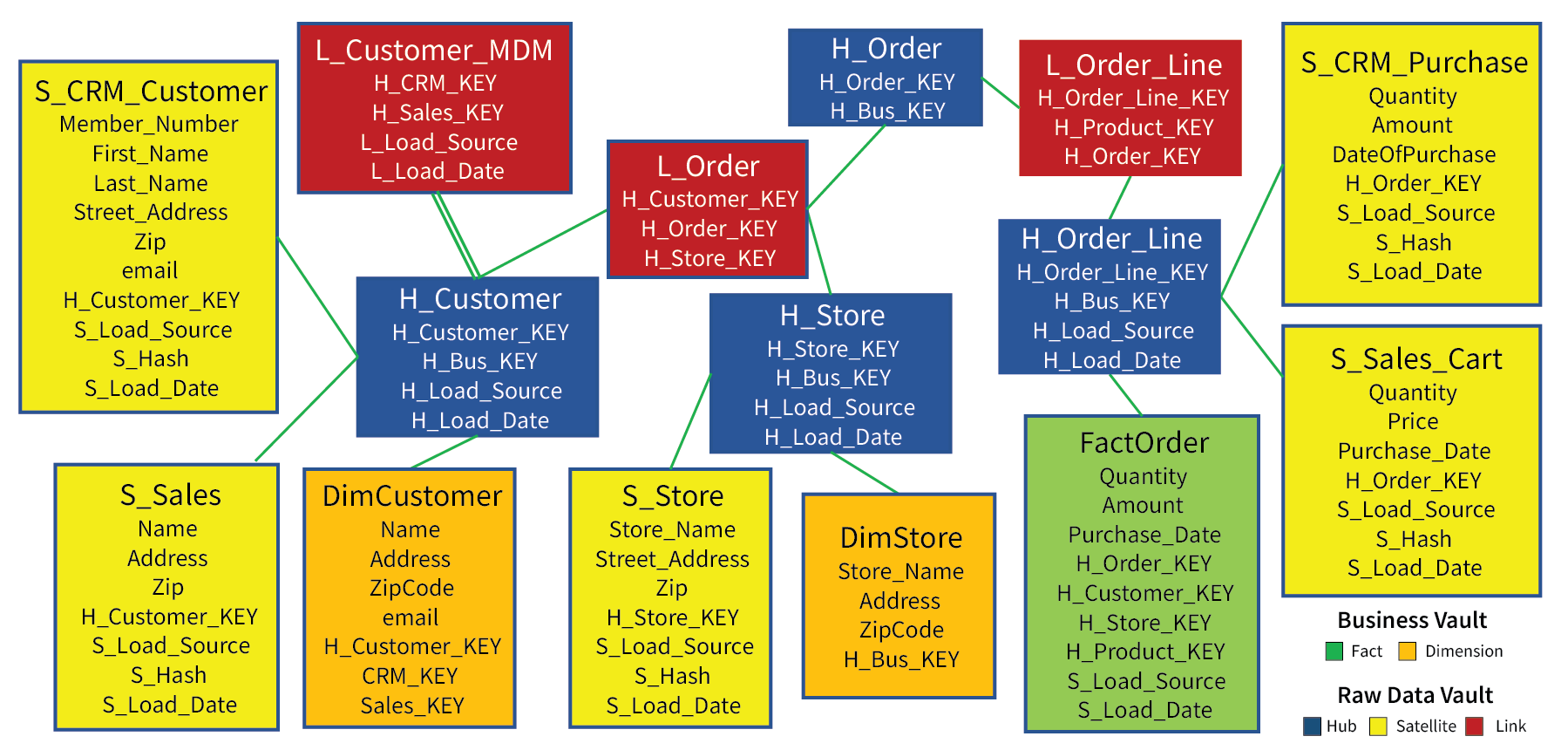
Figure 3 – Abridged view of a combined Raw and Business Data Vault.

Note that the dimension and fact tables are associated with a hub. The two dimension tables (orange) are normalized versions of the satellites under their respective hubs (blue). The fact table (green) is a union of the two Order Line satellites and associated with the H_Order_Line hub.

The L_Customer_MDM table is a special kind of link table known as a “Same As” table. In this case, it’s a Master Data Management table that holds mappings of the CRM customer to the corresponding Sales customer. It will be used to merge the satellites belonging to the CRM and Sales sources under the H_Customer hub into the DimCustomer table.

Customer Ensemble

Three of the four dimensions in our example are very straight-forward. The H_Store and H_Product hubs consist of just one satellite each, so there is no merging, morphing, and contorting involved with denormalizing those entities into dimension tables. H_Order_Line has two satellites, but we’ll address that when dealing with the fact table. So we’ll tackle the tough one, Customer with its four satellites, as the sole example of creating a dimension table. The same principles will apply to the other three dimensions.

Figure 4 illustrates the Customer Ensemble. Roughly speaking, an ensemble is a set of raw data vault tables directly related to a hub. In this case, Figure 4 includes Business Vault tables (orange) that are also related to the H_Customer hub. The four satellites, hub, and link are the raw material for what is needed to take us from the raw data vault satellites to the DimCustomer dimension table.

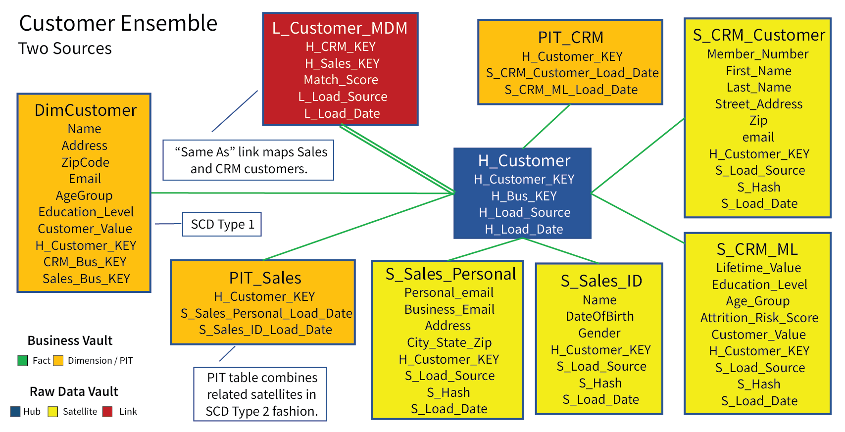
Figure 4 – The Customer ensemble.

Note that the MDM link table, L_Customer_MDM, is included in the Customer ensemble. As mentioned, its purpose is to match customers from the CRM system to their counterparts in the Sales system. For example, the CRM system may have a customer named “Eugene Anderson” and the Sales system may have “Eugene A. Anderson”. The L_Customer_MDM table holds a row asserting that they are the same person. This mapping ensures our DimCustomer table recognizes Eugene Anderson just once.

Regarding the two PIT tables, PIT_CRM and PIT_Sales. These are “Point-In-Time” tables, intermediary steps between the raw data vault tables and DimCustomer. The road from coherent satellites to integrated dimensions is sometimes a rocky one requiring several intermediary steps such as the formation of these PIT tables.

The following few topics describe the customer ensemble tables shown in Figure 4. For the sake of simplicity, I’ve inserted very minimal “toy” data to make my points.

Customer Satellites

Figures 5a-d, displays the toy data of the four satellites related to the customer hub. The names of the satellite tables follow the format of S__. For example, the breakdown for S_CRM_Customer is as follows:

• S – Indicating this is a satellite table.
• CRM – Concept. In this case, since the customer data comes from two sources, this indicates the source, CRM or Sales.
• Customer – Aspect. Some word symbolizing the column family.

Figure 5a shows two customers in the CRM system. Notice that Eugene shows up twice (on 10/15/2020 then again on 10/18/2020) due to a changed Street Address and Zip. Satellites are slowly-changing dimensions Type 2 (SCD Type 2) tables, retaining a history of “versions” for each hub entity.

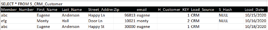
Figure 5a – S_CRM_Customer Satellite. Column family of basic customer information.

Figure 5b shows results for Eugene and Monty from four machine learning models developed by data scientists and operationalized in the CRM system. Again, Eugene shows up twice (once on 10/15/2020 then on 10/20/2020) since his Age Group and Customer Value rating changed. His original 60-70 age group was apparently a birthdate error and later updated, along with a new customer value rating.

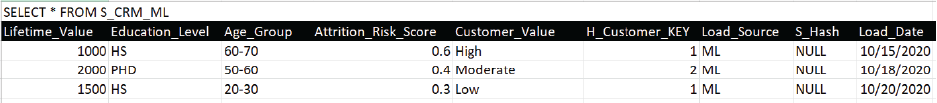
Figure 5b – S_CRM_ML Satellite. Column family of ML model outputs. The left four columns are output from 4 ML models.

Figures 5c and 5d are similar to the two previous Figures, but for the Sales source system. Figure 5c shows the required customer ID information for the Sales system.

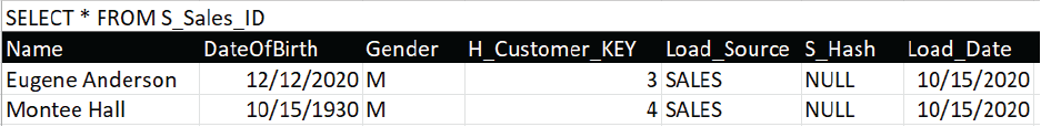
Figure 5c – S_Sales_ID Satellite. Column family of basic customer ID information from the sales Web site.

Figure 5d shows optional customer identification. It’s the typical sort of data only required when the user makes a purchase and so we need to know where to ship it.

Figure 5d – S_Sales_Personal Satellite. Column family of data required to ship a purchase.

Figure 6 shows data in the H_Customer hub table. Hubs are generally derivable from satellites. In our toy case, we show four entities, two each from the CRM and Sales systems. The hub does not reflect the multiple versions of each customer. That is the satellites’ job.

Note that the four satellites shown in Figures 5a-d join to H_Customer on H_Cutomer_KEY.

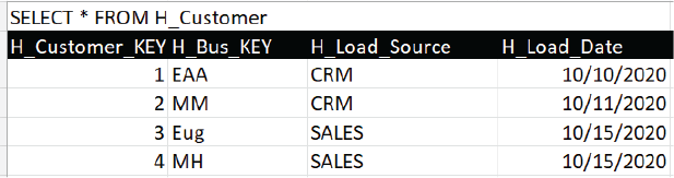
Figure 6 – H_Customer data.

Although the four rows in reality represents two unique people (EAA/Eug and MM/MH), the hub must recognize the entities as they are in the source systems. Remember, the value of the raw data vault includes:

1. 1. 1. The expediting of data into the “data warehouse” before the arduous task of hammering out master data mappings and/or value definitions.

2. Storing raw history so that we preserve data as is. We can transform and re-transform it in evolving ways from multiple points of view.

Note the H_Bus_KEY, the unique “business key” defined in the respective source system. The pair of H_Bus_KEY and H_Load_Source should form a unique key.

Customer MDM

Figure 7 shows the toy data in the L_Customer_MDM table. Each row maps customers from the CRM system to the customers/leads in the Sales system.

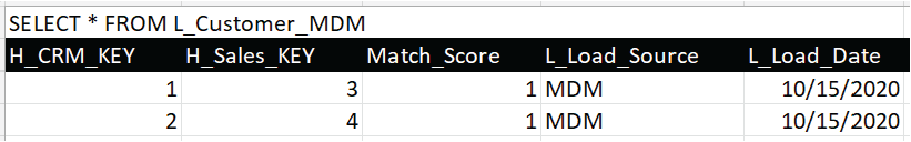
Figure 7 – L_Customer_MDM data.

Because data vaults hold data from different source systems, whether departmental or lines of business, master data management plays a very important part in the integration of data across multiple sources. Without the ability to map entities from source to source, the data is stuck in data silos.

MDM mappings are usually daunting tasks, especially for people-related entities due to the large number of people, common names, misspelled values, privacy issues, etc. MDM processes are usually sponsored by a Data Governance body. They involve the subject matter expertise of data stewards and the data wrangling expertise of data engineers and/or data scientists.

L_Customer_MDM is a specialized link table (“same-as” table). They are generally considered a business vault table since “mappings” are more like a rule than just data.

Customer PIT Tables

Point-in-Time (PIT) tables are a business vault table that denormalize satellites in two ways. The first is by setting effective date ranges. As mentioned, Data Vault satellites capture historic changes. In BI terms, every satellite is slowly-changing Type 2. The resulting PIT table holds a record for each “version” of the entity with the effective and expiration dates. With the PIT table we’re able to look back at what the state of each customer was at a given point-in-time.

The second is by merging satellites from multiple sources into one. Joins are compute intensive, especially when there are many satellites and/or very many rows.

Figure 8a depicts a sample of a very good pattern I long ago adopted from Dani Schnider’s blog for the creation of a PIT table.

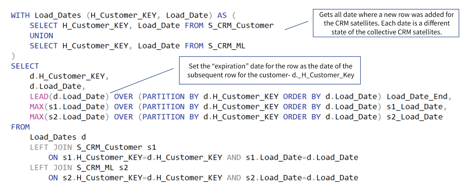
Figure 8a – SQL for creation of the PIT_CRM table.

Materializing the joins and computation of the date ranges in a PIT table preserves the time and cost of substantial processing that could be prorated over multiple consumptions.

Figure 8b depicts the result of the SQL in Figure 8a. This is our flattened SCD Type 2 PIT table for the CRM system.

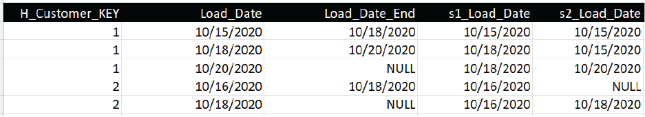
Figure 8b – PIT_CRM data.

Note the first three rows where H_Customer_KEY=1. The three rows means that data for customer key 1 changed twice. The first change occurred on 10/18/2020 in the CRM system. Looking back at Figure 5a, that’s when Eugene moved from Happy Ln to Happy St. The second change happened on 10/18/2020. Looking back at Figure 5b, it’s when Eugene’s age group was corrected from 60-70 to 20-30.

The most important characteristic of Figure 8b are the NULL values for Load_End_Date in the 3rd and 5th rows. These values are NULL because there are no superseding rows for the customer key. These are the “latest and greatest” versions of the two CRM customers. That’s an important thing to know for the SCD Type 1 DimCustomer dimension table we’re going to create.

Figures 9a and 9b are pretty much the same as 8a and 8b, but for the Sales system.

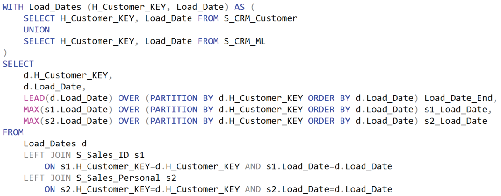
Figure 9a – SQL for the PIT_Sales table.

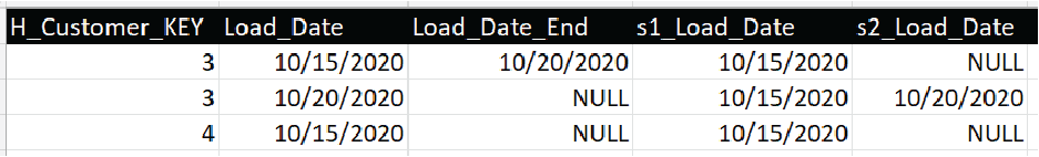
Figure 9b – PIT_Sales data.

DimCustomer

DimCustomer is the customer dimension of our toy star schema. It is the final product of the Customer Ensemble section. For the sake of simplicity, this will be a slowly-changing dimension Type 1 (SCD Type 1). That means only the latest version of the customer attributes are considered.

Figure 10a depicts the SQL for the creation of DimCustomer. Some points of interest include:

• The L_Customer_MDM table is the driving table. Each row represents the keys to one customer, but from two different sources (CRM and Sales).
• The WHERE clause filters for only rows where the Load_End_Date is NULL. This is the “flag” for the latest and greatest version. This WHERE clause would be eliminated if we were creating an SCD Type 2 dimension.
• The SQL expressions that are more than simply specifying a column in the SELECT list could be considered “business rules” defining transformation from one format to another.
• The joins are very straight-forward. This means that programmatic construction of this SQL is readily automatable by the data vault tool.

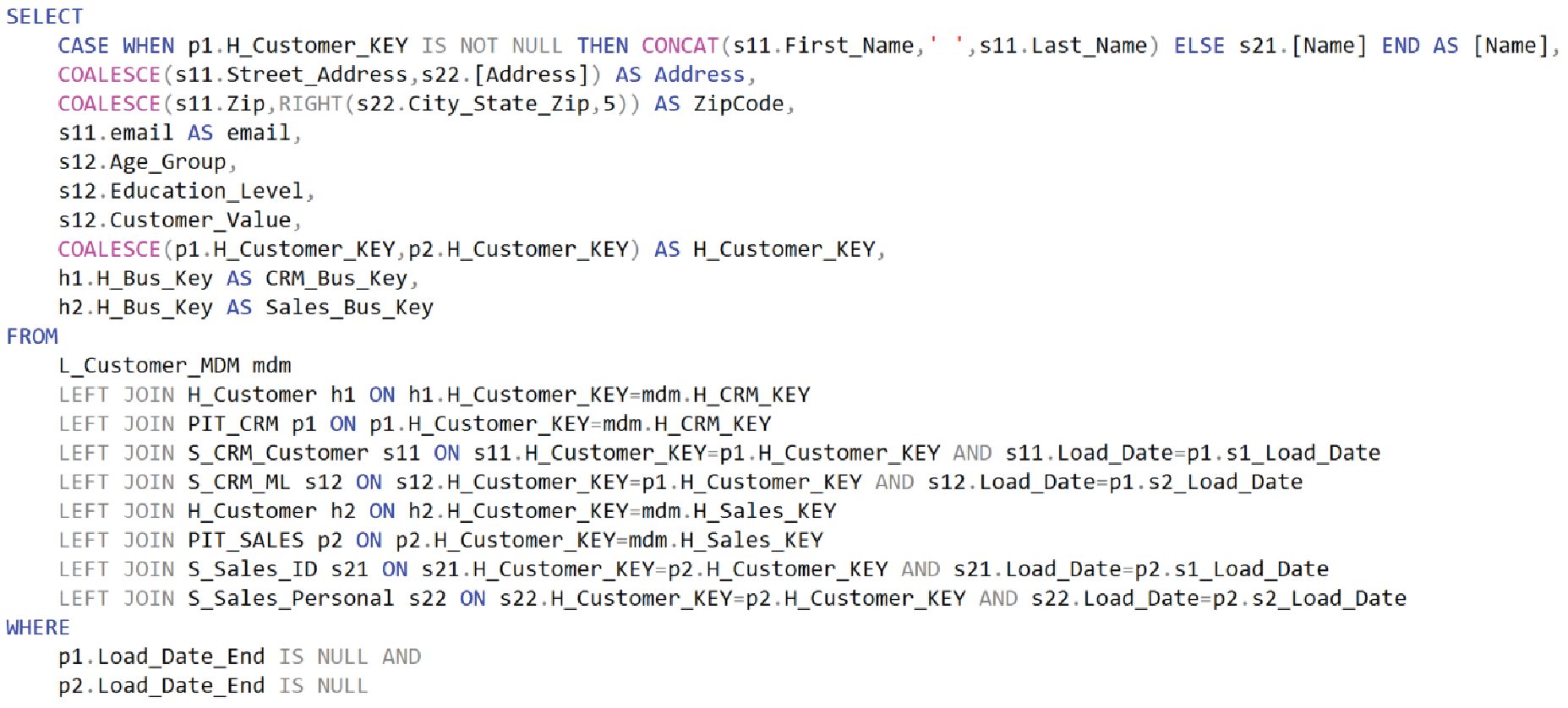
Figure 10a – SQL for the DimCustomer table. It’s an SCD Type 1 table.

Figure 10b shows the result of the SQL in Figure 10a. It returns one row of a mix of CRM and Sales attributes for each unique customer.

Figure 10b – DimCustomer data.

H_Customer_Key is the primary key for this table. Note that it is the H_Customer_Key for the CRM version of the customer. A subtle business rule implied in the Figure 10a SQL are in the COALESCE functions. That is, the CRM system is the “golden record”, the default value. The COALESCE statements say: Use the CRM value, but if it’s NULL, use the Sales value.

As to the question of whether we should materialize DimCustomer or treat it as an unmaterialized view, that depends in part on how many different times it will be used. Consider that there could be many different “customer dimensions” for various subject-oriented or departmental data marts and/or cubes. Each would probably consist of different columns of interest for different analyst needs across what could be a fair number of satellites. This notion of many customer dimensions stems from the E-L-T notion of “extract and load once, transform lots of different ways”.

For the most part, other customer dimensions would start with the same base: L_Customer_MDM, H_Customer, and the two PIT tables. But the selection of columns from satellites and the application of business rules would vary depending on need. There could be multiple PIT tables, depending on how many sources L_Customer_MDM maps and how many are involved.

Business Rules

Transformations are pretty much about the application of business rules. Examples of business rules include:

• Mapping – Match entities with different IDs but represent the same thing.
• Translation – Convert values into a common unit of measure.
• Formatting – How data is presented.
• Joins – How different satellites merge together.
• Filters and sets – Which rows are included in a business vault table.
• Calculations – Measure formulas.

Ideally, “rules” can be encapsulated as user-defined functions (UDF) as opposed to inline as shown in Figure 10a. Encapsulating rules in UDFs means the rule is constructed in one place. This is following the software development rule of DRY (don’t repeat yourself). Relational databases such as Snowflake, SQL Server, and Oracle have powerful features for authoring SQL Expression transformations and calculations.

However, UDFs should be applied only in the SELECT list. Using UDFs in the FROM or WHERE clauses can impede the ability of query optimizer to choose the best join strategy.

Very sophisticated calculations can be authored as Kyvos calculated members, encoded as MDX expressions.

• MDX is the language of cubes. Aside from possibly DAX, it’s unparalleled at expressing calculations in multidimensional space.
• Cube developers have the option of creating “custom” calculations – which lives downstream from the Business Vault.

Order Line Ensemble

The order line is the main event of our toy example. It is the subject of the fact table which is the centerpiece of a star schema. The columns consist of keys for various dimensions, measures, and a few pieces of fact-level data.

For our toy example, creation of the fact table is simpler than it is for DimCustomer. The satellites are only split by source – not by source and purpose-specific column families as it is for customers. And the master data issue is already resolved in the customer ensemble. FactOrderLine is simply a union of order lines from the CRM and Sales sources.

Figure 11 depicts the Order Line Ensemble.

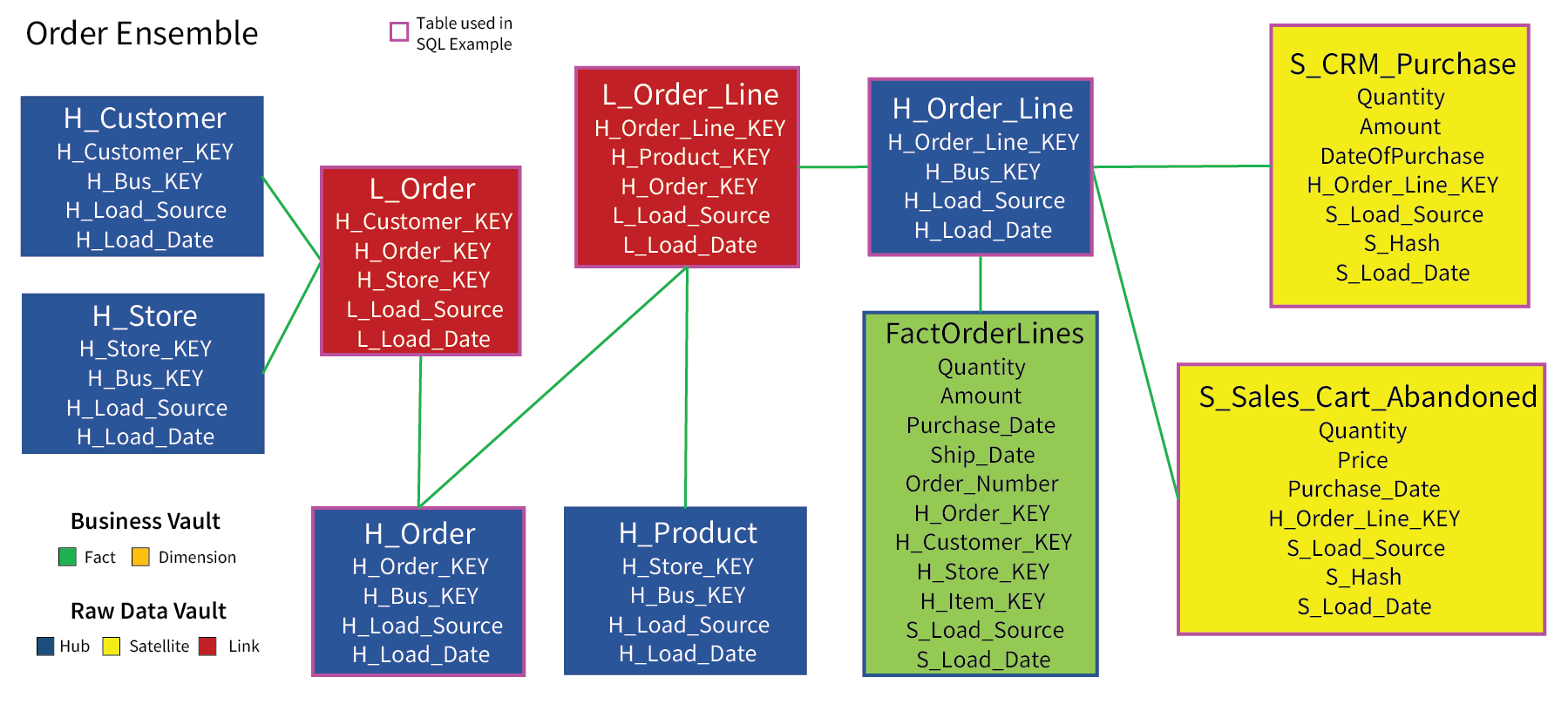
Figure 11 – Order ensemble.

The tables lined in magenta are the tables actually involved in the SQL that results in the FactOrderLines table. Figures 12a-g show the data in these tables.

The root of the order ensemble is the order. Each order has multiple order lines. Figure 12a shows that our toy example consists of two orders, one each from the CRM and Sales sources.

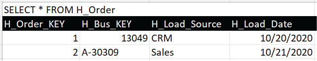
Figure 12a – H_Order, hub for the Orders.

Each order is associated with a customer and a store. Figure 12b shows the link table associating the orders with their respective customers and store.

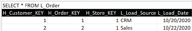
Figure 12b – L_Order, link table that ties the customer and store to the order.

Each order consists of one or more order lines, one for each product. Figure 12c is the hub for the order lines. Each of our two orders consists of two lines each.

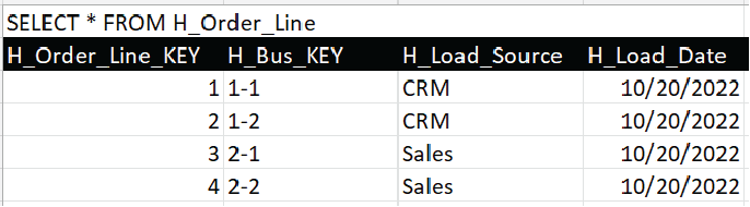
Figure 12c – H_Order_Line

Figure 12d is the link table that associates each order line to its parent order and the order line product.

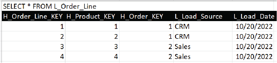
Figure 12d – L_Order_Line.

As is usually the case, the data “payload” is in the satellites. For our toy example, those are S_CRM_Purchase and S_Sales_Cart_Abandoned. Figure 12e and 12f shows two order line items each from the CRM and Sales sources, respectively.

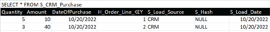
Figure 12e – S_CRM_Purchase.

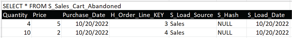
Figure 12f – S_Sales_Cart_Abandoned.

Now we’ll look at the SQL that will build the FactOrderLines table from those tables shown in Figures 12a-f. The FactOrderLines table is a UNION of the rows in S_CRM_Purchase and S_Sales_Cart_Abandoned.

Figure 13a depicts the top half of the SQL, the part that selects the S_CRM_Purchase rows.

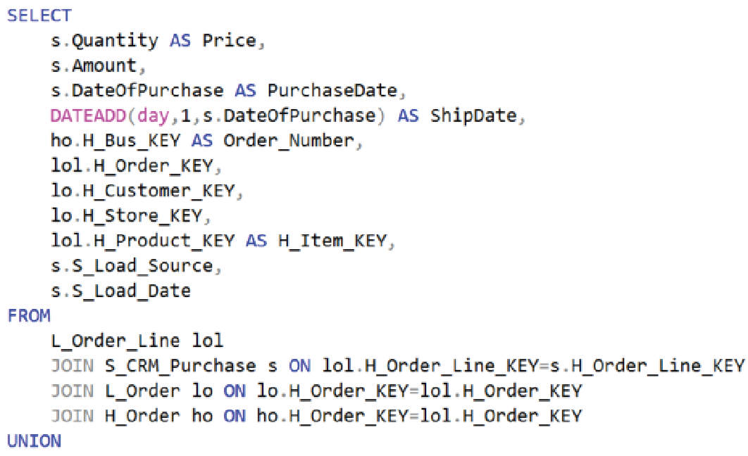
Figure 13a – First half of a SQL for the FactOrderLine table. Returns sales recorded in the CRM system.

Here are a few things to note:

• The joins are straight-forward, easily automatable using a data modeling tool.
• For the sake of simplicity, the ShipDate is just set to the day after purchase. In reality, an order could be shipped much later than the purchase date, which complicates matters beyond the scope of this blog.
• The first part of a SQL UNION statement dictates the column names.

Figure 13b below illustrates the second half of the SQL that creates FactOrderLines. In this toy case, the two parts are almost identical, with the major difference being the reference to their respective satellites.

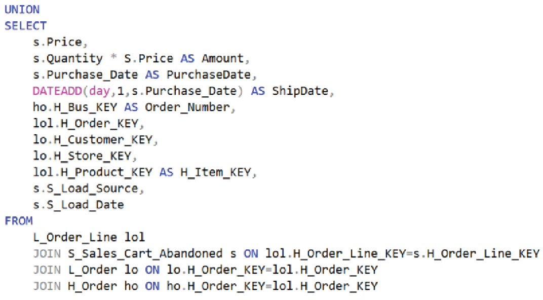
Figure 13b – Second half of a SQL for the FactOrderLine table. Returns sales recorded in the Sales system.

Figure 13c below is the result of the execution of the SQL that constructs the FactOrderLines table.

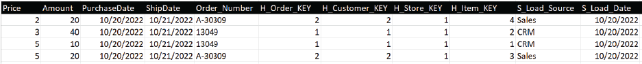
Figure 13c – The result of the SQL from Figures 13a and 13b.

Note that besides H_Customer_Key, there are foreign key columns linking to the order, store, and item dimension (H_Order_KEY, H_Store_KEY, and H_Item_KEY). As a reminder, we only covered the construction of the DimCustomer table. Construction of the other dimensions should be easy to figure out based on the explanation for DimCustomer.

The Kyvos Cube

With our dimension tables and fact table, we have a schema easily presentable to Kyvos. As a reminder, although we constructed a star schema, Kyvos can work with other formats including snowflake, flattened tables, and even 3rd normal form. We’ll address 3rd normal form in the next topic.

After configuring the connection information for the data vault in Kyvos, the next step is to register the files (as would be the case for S3, Hadoop, ADLS data sources) or table (Snowflake, Redshift). Figure 14 shows an example of defining one of those files/tables, FactOrderLines, in Kyvos.

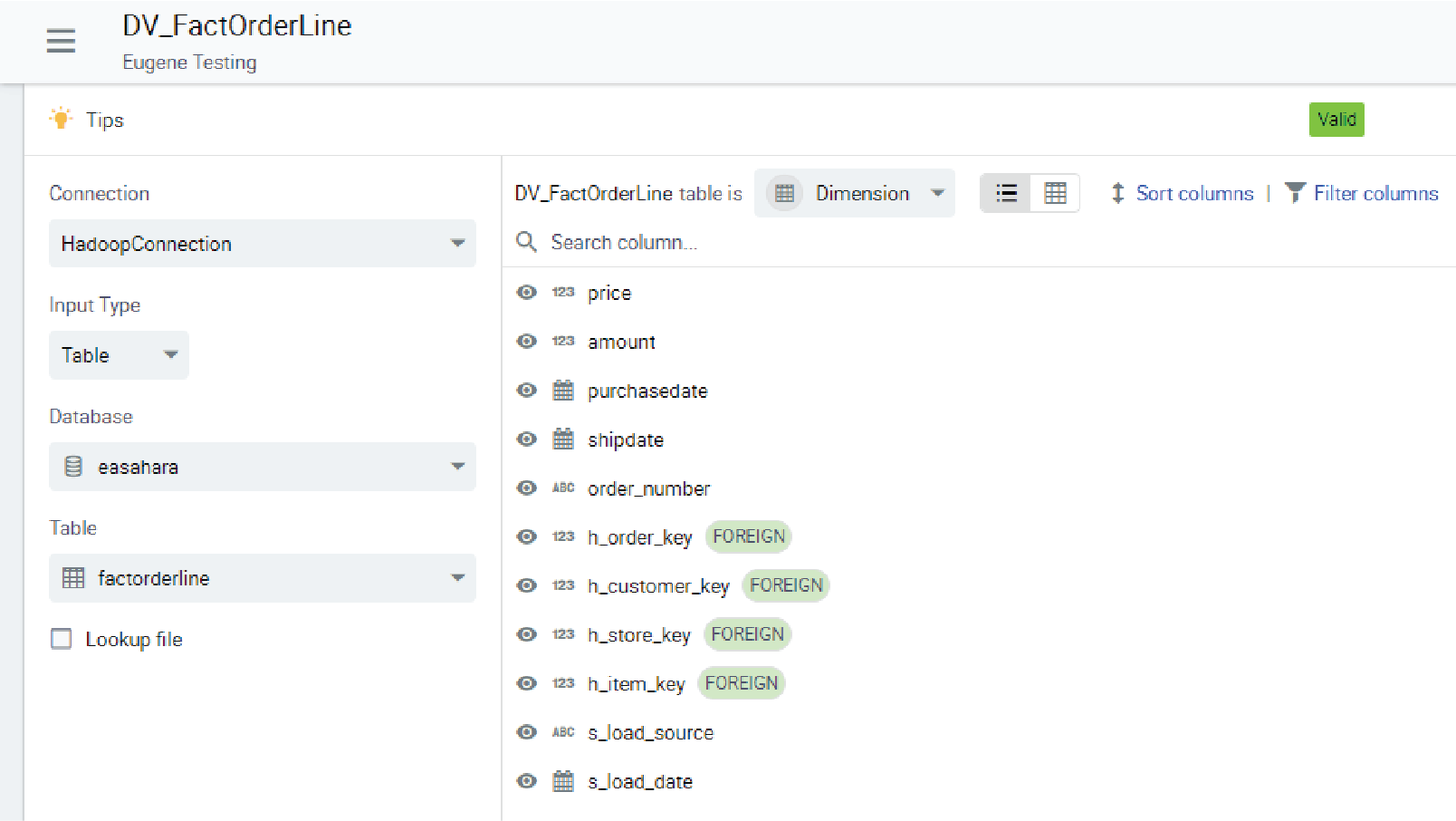
Figure 14 – The file definition for FactOrderLines.

Of course, we must also register file definitions for DimCustomer and the other dimension tables we didn’t specifically cover in this blog (DimStore, DimProduct, DimOrder).

We then construct a “Relationship” in Kyvos. For SQL Server Analysis Services fans, this is the same as the “Data Source View”. Figure 15 shows the star schema we build that will serve as the “source” of our Kyvos cube.

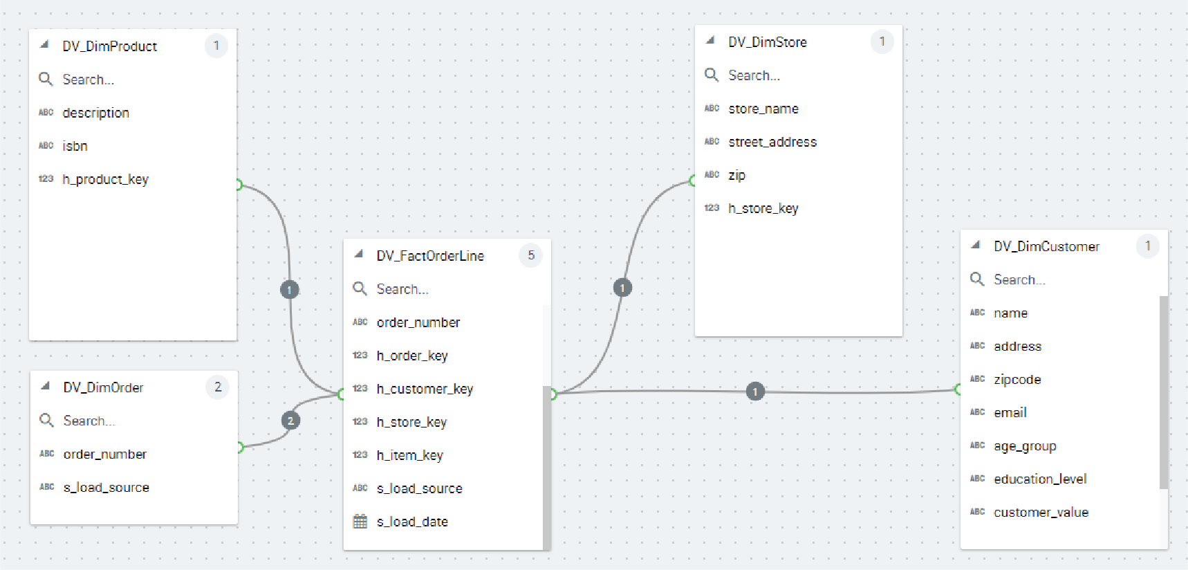
Figure 15 – Star schema designed as a Kyvos relationship.

Figure 16 shows the cube definition based on the star schema in Figure 15 above. Here, we see the role-playing dimensions for the Ship and Purchase dates, and dimensions defined for customer, store, order, and product.

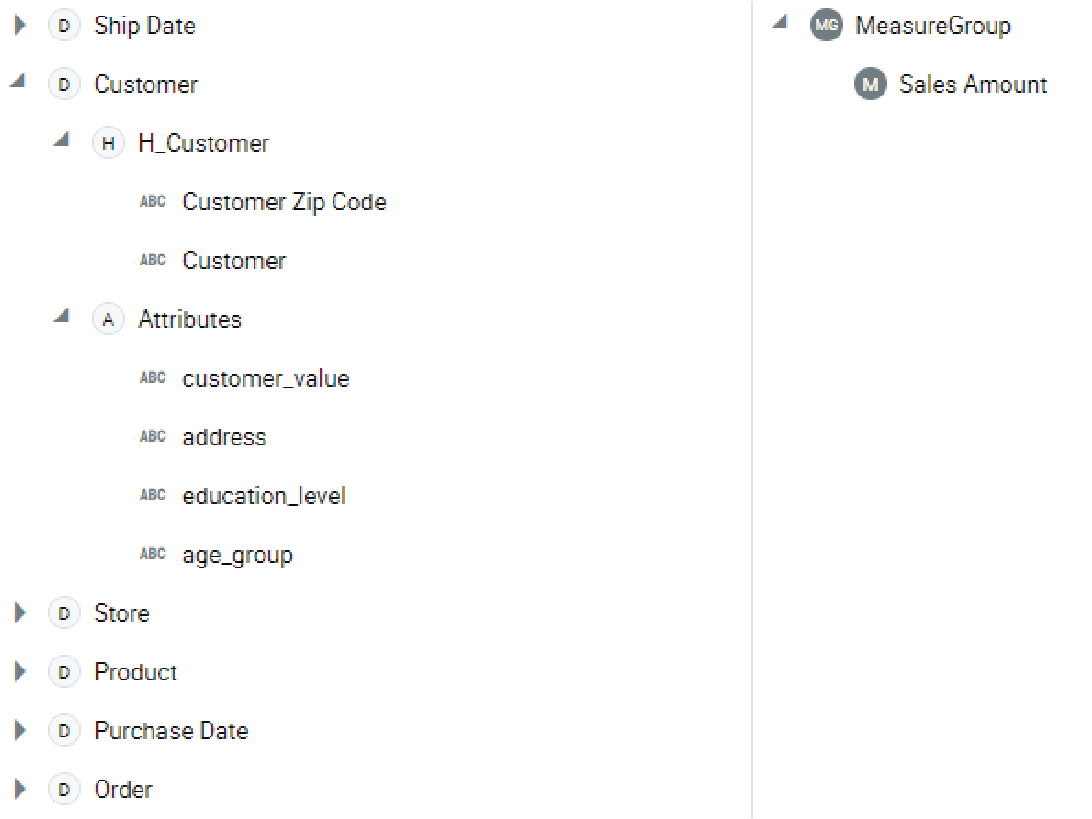
Figure 16 – Simple cube built from our business vault files.

Figure 17 below is a very simple report from the cube built in Kyvos with the data used in this blog.

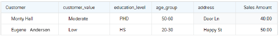
Figure 17 – Very simple report from the Kyvos cube.

Note that the values for age_group and address reflect the latest and greatest values for the customers since the customer dimension is SCD Type 1.

Kyvos SQL File Definition

Alternatively, Kyvos allows tables to be defined with passthrough SQL. That mitigates the need to materialize dimensions and fact tables in the data vault. This is very helpful if the data source is relatively complicated (ex. 3rd normal form) or further transformations are required.

Figure 18 shows how the DimCustomer SQL from Figure 10a would look in the Kyvos File UI. The joins are straight-forward. However, if the two PIT tables were not materialized, the SQL would be much more complicated. We would need to embed the SQL of the PIT tables into the DimCustomer SQL. Not only will the DimCustomer SQL be much uglier, but the query would be much slower at cube-processing time due to the complications of attempting to crunch everything at once.

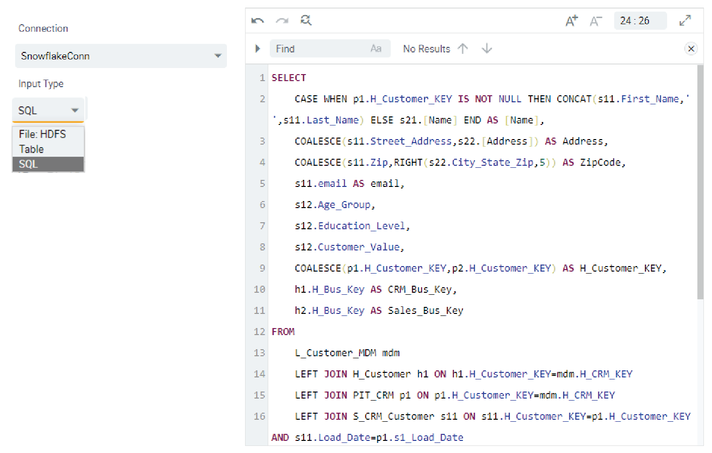
Figure 18 – Passthrough SQL Kyvos file definition. This is the same SQL for the DimCustomer table shown in Figure 10a.

Please note that although the choice of materializing DimCustomer in the Business Vault and again in the cube may be redundant storage-wise, as I mentioned earlier, it’s often the case that these business vault tables are used by more than one “client”. It’s possible that there are a number of departmental cubes, subject-oriented cubes, dashboards, reports, or Tableau users that might utilize this dimension table. By not materializing the table, the expensive compute is performed for each utilization.

Conclusion

In the E-L-T spirit of “load once, transform many ways”, the raw data vault is very attractive to those who just began investigating the Data Vault Methodology. It’s a versatile data warehouse structure that enables the expedited implementation of new data sources. However, in all that excitement, it’s easy to forget that there is a substantial gap between what is actually the raw data vault schema and the star/snowflake schema that facilitate user-friendliness and query performance. The Data Vault Methodology resolves this issue with the patterns of the Business Vault.

In the case of Kyvos’ OLAP cubes, those Business Vault objects comprise the dimension and fact tables of a star/snowflake schema. In this blog, we covered the more common patterns that move us from the versatility of the raw data vault to the streamlined structure of a star schema that presents a human-friendly semantic layer and magnitudes of performance optimization.