SSAS MD to Kyvos Migration – Part 3

This blog takes a mid-level dive into a comparison between the cube design experience of SQL Server Analysis Services (SSAS MD) and Kyvos Smart OLAP™. How does the experience differ? Why would aspects of cube design matter for SSAS MD, and why would it not matter in Kyvos? And what do we consider for Kyvos instead?

The hope is to answer the bulk of the questions you would have regarding an SSAS MD to Kyvos migration. This is the last blog of a 3-part series:

• Part 1: Cloud-based OLAP Solution. This series begins with a comparison of the high-level architecture of SSAS MD and Kyvos.
• Part 2: Overview of the Primary Objects. A comparison of the main parts of an SSAS MD and Kyvos implementation.

Please note that this blog:

• Is written for architects and developers responsible for technical evaluation.
• Assumes some experience with SSAS MD.
• Has a prerequisite of reading Part 1 and Part 2.
• Is not a tutorial on how to build cubes with Kyvos. If you simply wish to test drive Kyvos and migrating from SSAS MD isn’t applicable, please contact us for information on a free trial.

It’s important to note that although it may seem as if SSAS MD can sometimes seem more feature-rich than Kyvos, many of those features aren’t relevant in the Cloud-based world of Kyvos. Most of those features are geared towards performance tweaks within the less flexible hardware constraints of the SMP world into which SSAS was born. Because of the readily scale-out nature of Kyvos as well as the cloud in general, performance improvements are often a matter of simply adding more nodes.

The result is that the complexity of configuring and maintaining cubes is significantly reduced with Kyvos. Regardless, there’s still value in understanding the SSAS design decision points to ensure requirements reflected in the SSAS MD cubes are not lost in the migration.

Cube Design Experience

The Kyvos cube design experience should be fairly easy for an SSAS MD developer to pick up as it parallels the SSAS MD experience fairly well. But there are differences.

Table 3-1 maps the major pieces of the SSAS design process and the Kyvos counterparts. The numbers next to each item correspond to markers in Figure 1a illustrating the SSAS MD steps and Figure 1b illustrating corresponding steps in Kyvos.

The following table lists the objects that we’ll cover.

SSAS (Match Figure 1a numbers)	Kyvos Counterpart (Match Figure 1b numbers)
1-Server, 2-Instance, 3-Database	1- Account
4-Data Sources	2-Connections
5-Data Source View	3-Files, 4-Data Sets, and 5-Dataset Relationship Diagrams
6-Dimensions, 7-Cube	6-Dimensions and Cube Design are merged
8-Measure, 9-Partitions, 10-Aggregations	7-Partition and Aggregation Strategy

Table 3-1 – Cube design process

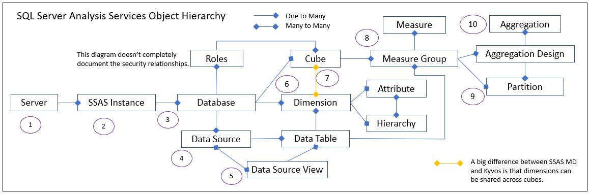
Figure 1a – Hierarchy of the major SSAS objects. The numbers correspond to items under the SSAS column in Table 3-1

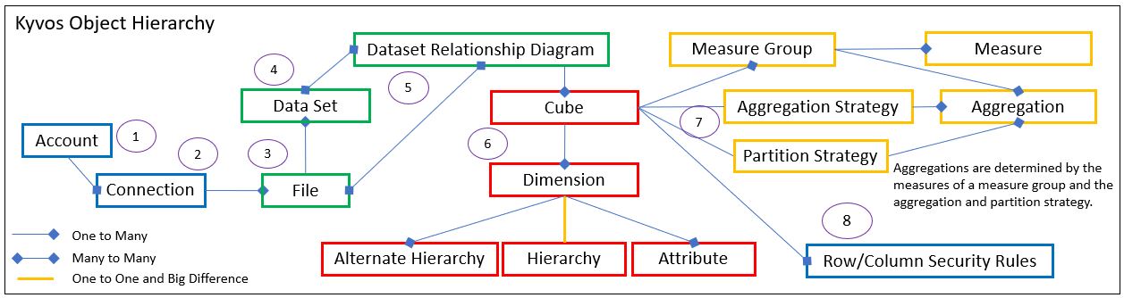
Figure 1b – Hierarchy of the major Kyvos objects. The numbers correspond to items under the Kyvos column in Table 3-1.

Figure 1b shows Kyvos broken into three groups of objects signified by color:

• Green – These Kyvos objects equate to the SSAS MD Data Source View (DSV).
• Red – These are the objects that comprise the cube and dimension relationship.
• Yellow – Measure groups and aggregations.

The red grouping in Figure 1b is intended to elaborate on the yellow line in Figure 1a between Cubes and Dimensions. SSAS MD dimensions are shared across multiple cubes in an SSAS MD database. But in Kyvos, cubes have their own dimensions. The red and yellow items in Figure 1b comprise what is configured through the Kyvos Cube Design UI.

The Cube Design Toolset

This blog includes snapshots from the SSAS MD and Kyvos design UIs. So before diving into the cube design experience, I need to briefly mention the source of these snapshots. SSAS’s toolset includes:

• Visual Studio-based BIDS development environment.
• SQL Server Management Studio for administration.

Kyvos development and administration is through a Web UI. As with SSAS, there are APIs for performing deployment and administration tasks. For SSAS MD, there is XMLA, AMO, and ADOMD. Kyvos includes XMLA and REST APIs.

Server, SSAS Instance, Database

One or more SSAS instances is installed onto an SMP server. A number of databases can exist on a single SSAS instance. In Kyvos, there is just Account. For each Account, there is a cluster of BI Servers, a cluster of Query Engines, a Cube Build cluster, and Cloud storage. All of the Kyvos items are configured with the customer’s Cloud environment (ADLS, S3, GCP).

Data Sources

SSAS “Data Sources” are analogues to Kyvos “Connections”. Figures 2a and 2b show examples of how SSAS Data Sources and Kyvos Connections, respectively, are set up.

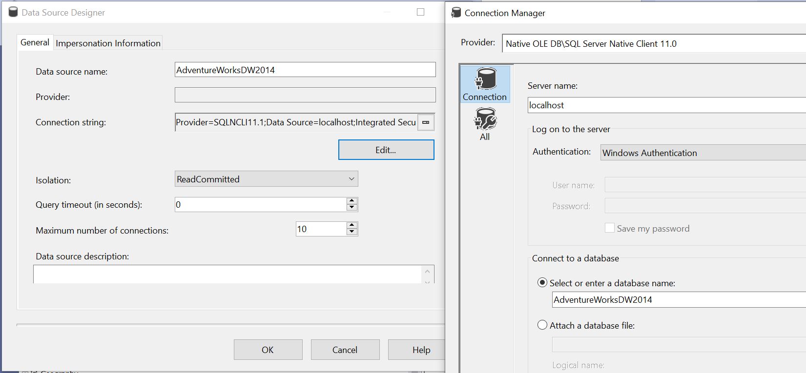
Figure 2a – SSAS MD Data Source. A typical SQL Server database via OLE DB.

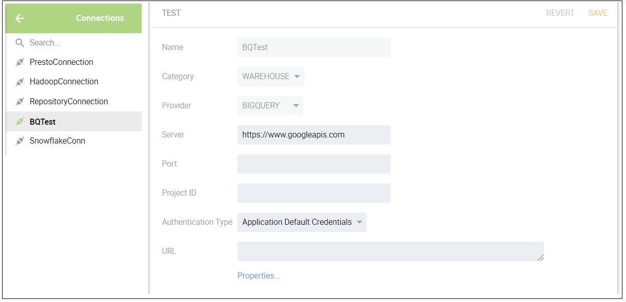
Figure 2b – Kyvos Connection.

SSAS MD and Kyvos both allow the configuration of multiple data sources. SSAS MD allows cubes to be created from dimensions and measure groups from different data sources, with some restrictions. For Kyvos, all cube objects must be sourced from one connection.

Roughly, data sources differ for SSAS MD and Kyvos in that for SSAS MD’s data sources are primarily relational databases (mostly SQL Server and Oracle), and Kyvos’ are Cloud-based databases.

The primary connection sources for Kyvos fall into a few categories:

1. Native Cloud Storage – AWS S3, Azure Data Lake Storage.
2. Data Warehouse – Snowflake, AWS Redshift. On the surface, it acts like a relational database.
3. Google Cloud Platform. A wide, flattened table.

For other types of data sources, the workaround is to dump the data into a cloud storage account, such as AWS S3 or ADLS, which places it into the Native Cloud Storage category.

Data Source View

The SSAS Data Source View (DSV) is basically an Entity Relationship Diagram (ERD) constructed from tables from one or more Data Sources. It is an abstraction layer, a star/snowflake schema view translated from the data sources to the cube. The Kyvos analogue is the Dataset Relationship Diagram (DRD).

Figures 3a and 3b show samples of the UIs for SSAS’s DSV and Kyvos’ DRD, respectively. The primary function performed within both UIs is to relate tables into a star/snowflake schema with PK/FK relationships.

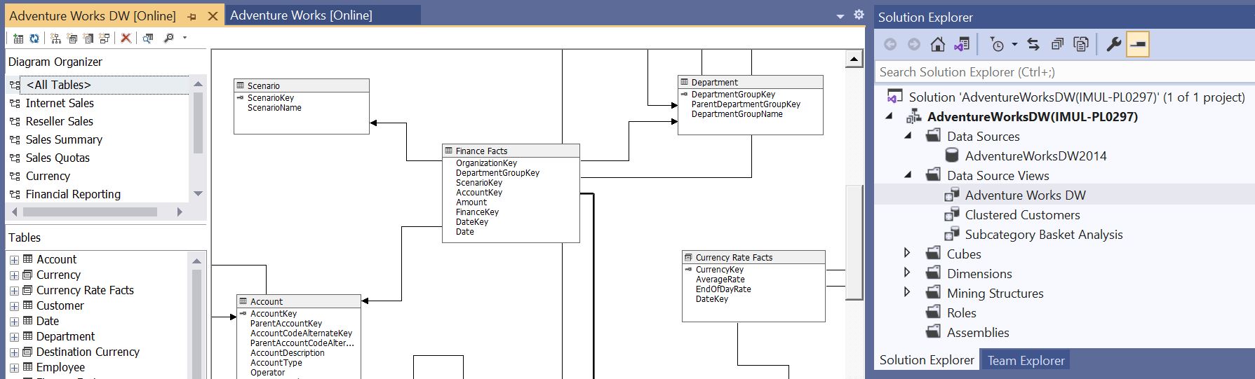
Figure 3a – An SSAS MD Data Source View. AdventureWorksDW is already a snowflake schema DW, so the DSV pretty much reflects the one data source.

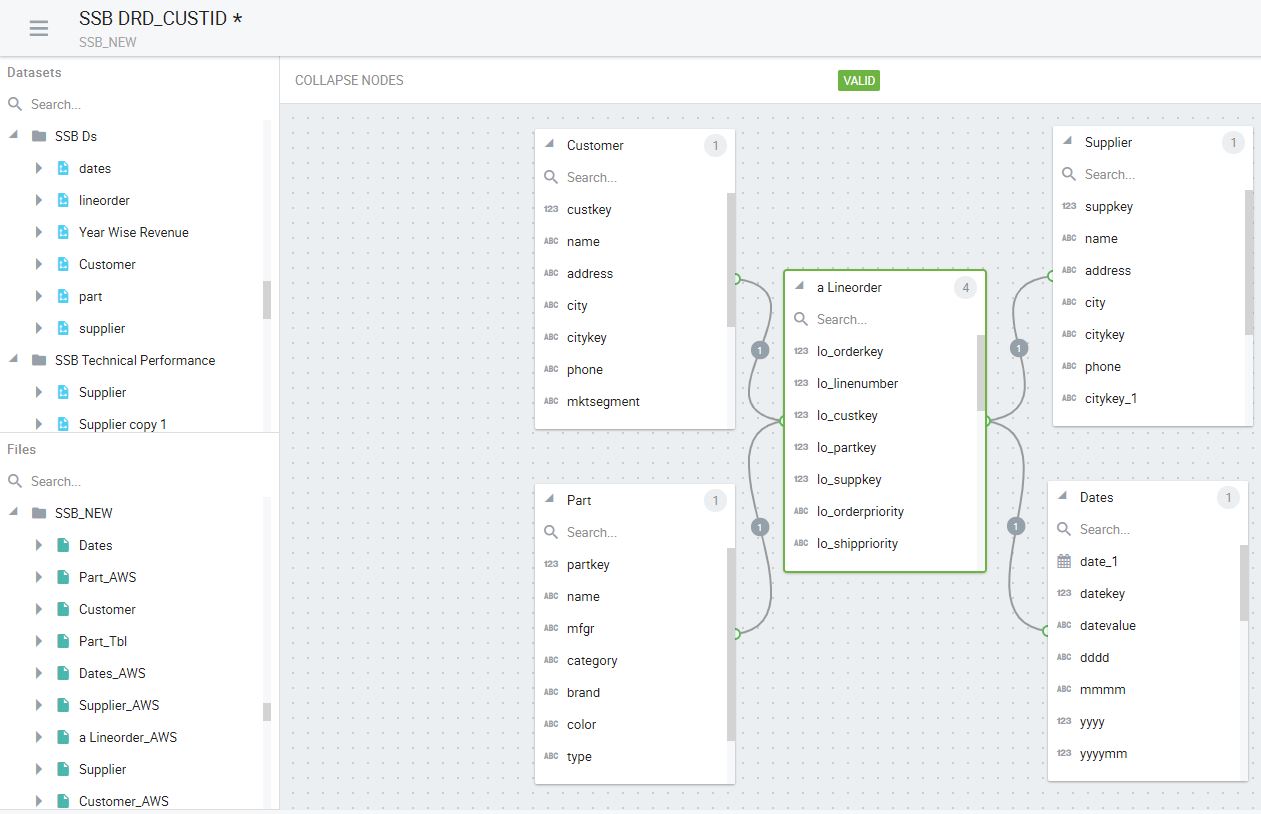
Figure 3b – Kyvos Dataset Relationship Diagram (DRD).

However, there are two major differences between the DSV and DRD depicted in Figures 3a and 3b:

1. For SSAS MD, light transform features are available in the DSV UI, but transform features for Kyvos are performed in steps prior to the DRD, which leads to point #2.
2. The data tables selected into the SSAS MD DSV are based on the tables and views directly from the Data Source (SSAS data sources are relational databases). Whereas for Kyvos’ DRD, the “tables” are Files and/or Datasets, before the DRD stage.

Notice on the left of Figure 3b, Datasets and Files are available to be selected as part of a Dataset Relationship Diagram. Way back in Figure 1b, we can see that Datasets are made of Files, and Dataset Relationship Diagrams are made up of Files and Datasets.

Table 3-2 lists SSAS DSV concepts, including the light transform capabilities in the DSV UI mentioned point #1, mapped to the Kyvos equivalent.

SSAS DSV Concept	SSAS DSV Concept Description	Kyvos UI
Data Table	Table or view from a data source.	File (Table/SQL), and/or Datasets
Named Query	Define a table with SQL	SQL and/or Datasets
Named Calculation	Define a column with a SQL expression.	SQL expr and/or Datasets
Friendly Name	Specify a friendly name.	SQL alias and/or Datasets
Data Relation	Relationships (lines linking the tables).	Dataset Relationship Diagram

Table 3-2 – Data Source View object comparison

For SSAS MD, the vast majority of ETL is performed prior to and outside of SSAS MD. In the SSAS world, that ETL tool is primarily SQL Server Integration Services (SSIS). SSIS packages extract from OLTP data sources, perform transformations, and load into a data warehouse, which is configured in our SSAS MD project as a data source.

Kyvos’ substantially more robust transformation capability results in a two or three-step process from Connections to DRD:

1. Files are created from tables (Snowflake, Redshift, Hive) or SQL based on tables in that Connection “registered” into Kyvos.
2. Data Sets – This is a built-in, versatile ETL feature. Files are munged with other files, transformations are computed, and a data set (like a table) is output.
3. Relationships – Files and/or datasets are configured into an ERD through the DRD UI depicted in Figure 3b. At this point, we have the Kyvos equivalent of an SSAS DSV.

It’s important to note that although the Data Sets feature is rather robust, DRDs can be constructed from Files alone. Heavy ETL processing should be performed outside of Kyvos with a dedicated ETL tool.

A Kyvos File is most like a DataTable in an SSAS DSV. However, it is often the case that the data we want doesn’t exist as a tidy table. For example, if the data source is Google Big Query, the dimensional model we want for our cube must be derived from one Big Table. Or, some data sources don’t have the concept of views as there are in relational databases. Therefore the SQL defining the File plays that role.

Kyvos’ Files defined with the SQL input type are like SSAS’s Named Queries. They are a means to specify a tabular structure as a SQL statement. The underlying data is transformable through SQL Expressions in the SELECT list.

As mentioned, substantially more robust transformations can be made using Kyvos’ Dataset functionality. Figure 4 shows a sample Dataset as a series of transformation steps from the file named “lineorder” to a Dataset named “Year Wise Revenue” (as shown in Figure 3b) accessible from a cube. It should be very reminiscent of an SSIS Data Flow.

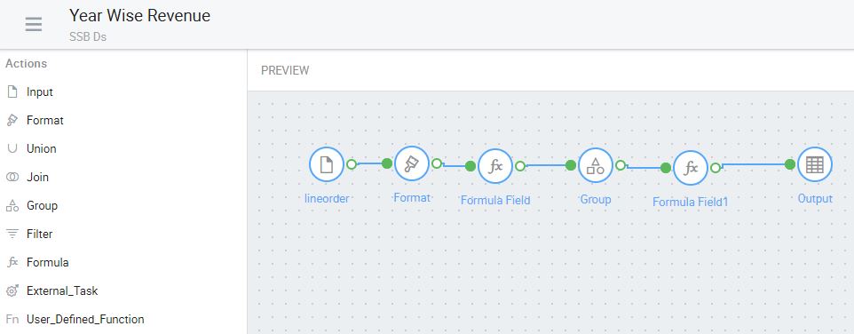
Figure 4 – A Kyvos Dataset. Substantial transformations can be designed within the Kyvos environment.

After Connections, Files, and Datasets are configured, we finally reach the point where we construct the Dataset Relationship Diagram. This involves dragging Files and/or Data Sets into a pane and setting relationships, similar to how DSVs are set up. See Figure 3b.

Cube Design

The Cube design experience maps fairly well between SSAS and Kyvos. The primary cube design difference is that for SSAS MD, the dimensions are database-level objects sharable by one or more cubes. For Kyvos, dimensions are designed at the cube level, therefore, unique to each cube.

The result of Kyvos cubes owning their own dimensions is that what is spread out among several UIs in SSAS MD is in one Cube UI for Kyvos. Table 3-3 lists the aspects of the SSAS MD cube design and the corresponding BIDS UI.

Cube Term	SSAS BIDS UI	Kyvos Cube UI Tab
Dimensions	Dimension	Design
Strong/Natural Hierarchy	Dimension	Design
Calculated Members	Calculations (MDX Script)	Design
Measure Groups	Cube Structure tab of the Cube window	Design
Measures	Cube Structure tab of the Cube window	Design
Calculated Measures	Calculations (MDX Script) tab of the Cube window	Design
Partitions	Partitions tab of the Cube window	Refine
Aggregations	Aggregations tab of the Cube window	Refine
Dimension MOLAP/ROLAP	Dimension	Design
MOLAP/ROLAP/HOLAP	Partitions	Design

Table 3-3 – Mapping of cube terms to the cube design UIs of SSAS MD and Kyvos. The Kyvos Cube UI Tabs are highlighted in the red box on Figure 5b.

What isn’t included in Table 3-3 is the Dimension Usage tab in the Cube UI (covered later on). SSAS MD allows for some modification of the link between dimensions and cubes. In Kyvos, all relationships are set at the DRD stage.

Figures 5a and 5b convey that the Cube Structure tab in BIDS is the closest analogue to the Kyvos’ Cube Design UI.
As mentioned, Table 3-3 shows the Kyvos Cube UI covers a wider range of the cube design experience. The big difference is that in the SSAS Cube Structure UI (Figure 5a), shared, database-level dimension are assigned to a cube. That’s opposed to how the dimensions are created in the cube design UI.

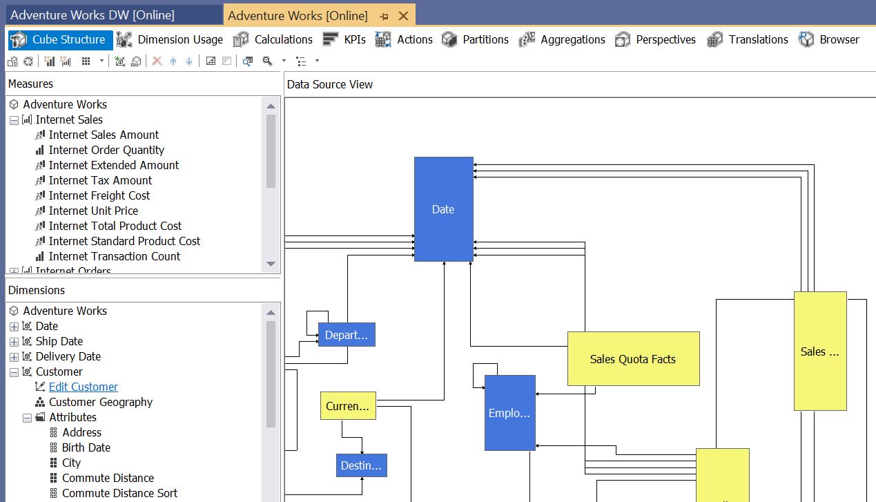
Figure 5a – SSAS MD Cube Structure. Notice the tabs along the top, which were mentioned in Table 3-3.

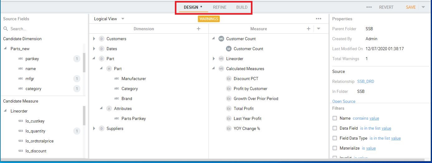
Figure 5b – Kyvos Cube Design UI. Notice the buttons in the red box, which were mentioned in Table 3-3.

The separation of dimensions and cubes in SSAS MD (database-level dimensions shared by multiple cubes) addresses two issues:

• Minimizing dimension and cube processing dependencies. Dimensions could be updated (new members and non-key SCD Type 1 changes) independently without forcing measure group processing.
• Minimizing DRY (Don’t Repeat Yourself)
  • Multiple cubes could use the same dimension, so multiple copies of the same dimension doesn’t need to be modified.
  • Dimensions could be used multiple times in the same cube as role-playing dimensions.
  • A dimension could be attached to another dimension as a reference dimension.

There are several reasons for having multiple cubes:

1. Cubes may have different processing requirements. For example, one may need to re-process daily, one monthly.
2. Targeted cubes could fit into memory. This was helpful if data is mutually exclusive. This improves concurrency.
3. Simplification of a cube for the end users. Although simplification for the end user can be handled with SSAS perspectives, simpler cubes are easier for developers to maintain.

The horizontally scalable Cloud nature of Kyvos ameliorates and often removes the first two reasons that lead to multiple cubes. Large cubes could be scaled out over more servers (see Part 1) as necessary to meet responsiveness and concurrency requirements.

Cube Design Wizard

SSAS’s “Cube Design Wizard” is usually used to build a first draft of a cube. In the wizard, the user selects a DSV, fact tables, dimensions, attributes of the dimensions, and measures. Valid options are determined at each step by relationships set in the DSV. Upon completion of the selections, in a single process:

1. The dimensions (shared by all cubes in the SSAS database) are created.
2. A cube object is created.
3. The selected dimensions are assigned to the cube.
4. Default measure groups and measures are added to the cube.
5. Default relationships (based on relationships in the DSV) are set.

The wizard does a really good job at that first draft of the cube. But there are generally manual tweaks to all of the objects – the dimensions, cube, measures, dimension, and fact table relationships – that could be subsequently performed.

I don’t recall anyone not starting off development of an SSAS cube in this manner. In fact, it was common for the Cube Design Wizard to perform almost all of the work, saving the developer from the advanced aspects of SSAS. However, many of those advanced issues raised its ugly head in the future, triggered by scale or new data issues.

Kyvos recently released a feature similar to the Cube Design Wizard that will likewise streamline the cube design experience. This wizard combines elements of the Data Source View Wizard and the Cube Design Wizard. It will be a 4-step process: Register Files, Define Relationships, Design Cube, Review and Build.

Dimension Usage Tab

The SSAS Dimension Usage tab features a matrix for setting how dimensions relate to measure groups. Most of the settings in this tab are automatically set, based on relationships set in the DSV, by the Cube Design Wizard, or changes to measures and/or dimensions in the Cube Structure tab. However, there are settings that may need to be manually set:

1. Changing the granularity of a relationship between a measure group and the dimensions.
2. Setting Reference, Many to Many, or Fact relationships between measure groups and dimensions.
3. Changing the keys that link the measure groups and dimensions. For example, for role-playing dimensions.

As mentioned earlier, Kyvos doesn’t have an equivalent of the Dimension Usage tab. All relationships are set in the Data Relationship Diagram, upstream of the cube design step.

Measures and the MDX Script

For SSAS MD, once the dimensions and measures are selected, the next step is to add globally-scoped calculated measures, calculated members, overlays for scopes of cells, and sets of members. This set is called the MDX Script and is configured using the Calculations tab (3rd tab from the left in Figure 5a).

As mentioned in Part 2, Kyvos doesn’t have a centralized globally-scoped MDX script. However, most of what is configured in the MDX script exists elsewhere for Kyvos, as shown in Table 3-4

MDX Script Item	Kyvos Equivalent
Calculated Member	Calculated Member configured with dimension attribute.
Calculated Measure	Calculated Measure configured under Measure Group.
SCOPE	Convertible into conditional MDX.
STATIC SET	Session and Query-scoped only. Global-scoped on roadmap.
DYNAMIC SET	In evaluation for roadmap.

Table 3-4 MDX Script item comparison

Cube Refinement

With this section, we’re exiting from what is strictly “cube modeling” into the cube refinement aspects of partitions and aggregations. The challenge in describing these two complicated and highly technical topics is that they go hand in hand. So I need to explain them together. That’s true for both SSAS MD and Kyvos.

Following is a high-level description of these relationships between partitions and aggregations:

SSAS MD:

1. Measure groups are partitioned into horizontal chunks, for example, by year.
2. Each of those partitions can be assigned one of the multiple Aggregation Designs created for that measure group.
3. Each of those partitions can be stored in MOLAP, HOLAP, or ROLAP mode.

Kyvos:

1. Each aggregation is distributed to a hash-determined Query Engine node.
2. The aggregations are partitioned into chunks and stored as separate files on the aggregations’ assigned Query Engine node. For example, by year.

MOLAP, HOLAP, and ROLAP

Before discussing Partition and Aggregations, we need to discuss OLAP storage modes for the cube objects. For SSAS MD, these storage modes are a factor in the partition and aggregation design.

Table 3-5 compares the meanings of MOLAP, HOLAP, and ROLAP for SSAS and Kyvos. For both SSAS and Kyvos, Dimension and Measure Groups can be MOLAP or ROLAP. However, HOLAP has different meanings in SSAS and Kyvos.

Storage Mode	SSAS	Kyvos
MOLAP	Dimensions and Measure Groups are all processed.	Same.
HOLAP	Dimensions and Measure Group Partitions.	Mix of MOLAP/ROLAP Dimensions and Measure Groups.
ROLAP	Dimensions and Measure Group Partitions.	Dimensions and Measure Groups.

Table 3-5 – MOLAP/HOLAP/ROLAP comparison.

MOLAP is the most performant for both products. For MOLAP, dimensions, aggregates and the “fact level data” are processed and stored in the SSAS MD or Kyvos storage environment. The design considerations for MOLAP include:

• Extra storage cost for the SSAS MD MOLAP objects. Storage cost is less of an issue for Cloud-based Kyvos storage.
• Is there a real-time requirement? If latency (in the range of days or hours) isn’t acceptable, MOLAP isn’t an option. ROLAP will be required to access the latest data on the underlying data source.

The MOLAP cube process for fact tables is similar for both products:

1. The fact data is read from the data source and a lowest-granularity data object is created and stored. The underlying data source is touched only at this time. For Kyvos, this is called the “root cuboid”. For both products, it is the largest data object since it’s at the lowest granularity.
2. Aggregations are generated from that lowest-granularity data object.
3. For SSAS, indexes are built for those aggregations. This doesn’t apply for Kyvos’ Cloud storage.

ROLAP is the least performant since queries are resolved at query-time from the underlying data sources. The primary design considerations are:

1. The price for unpredictable and excessive load on the OLTP data sources and the resultant network delay in exchange for up-to-date data (the data source is usually in a different environment).
2. Unpredictable OLAP query performance since the state of the underlying data source is out of the control of the OLAP system.
3. No pre-aggregation of data, which results in savings on the storage cost of MOLAP data.

For SSAS MD, HOLAP means that for a measure group, aggregations are created and stored in the SSAS environment. But the lowest-level facts are not copied over. So if a requested aggregation doesn’t exist, SSAS will query the underlying data source on-the-fly at query time. This works well when the attributes involved in the queries are known. We then can design the aggregations that cater to those known combinations of attributes.

For Kyvos, HOLAP means that dimensions and measure groups of a cube can be a mix of MOLAP and ROLAP. For example, a measure group may contain prices that change frequently. This measure group could be set as ROLAP. Current prices would be read at query-time from the up-to-date, underlying data source.

Partitioning

This topic and the next (Aggregation Design) are about parallelization of cube processing and query processing. The concept of parallelism in relation to SSAS and Kyvos has several meanings. Table 3-6 lists the types of parallelization covered in this topic.

Parallelism Category	SSAS MD	Kyvos
Storage of Data	Specification of storage device per partition	Cloud Storage – sharded across many servers
Reading Data from storage	Thread per partition on one SMP reading from multiple storage devices	Threads across a cluster of Query Engine nodes
Query Processing	Threads on one SMP	Threads across a cluster of Query Engine nodes
Cube Processing	Thread per partition on one SMP	Distributed across a Spark cluster

Table 3-6 – Parallelism. In a nutshell, SSAS MD is limited to threads on one SMP and Kyvos processing is parallel across many Query Engine nodes.

For SSAS MD and Kyvos, partitioning and aggregation go hand in hand. That’s because it is aggregations that we’re partitioning. However, partitioning has different meanings in the SMP world of SSAS MD and the Cloud world of Kyvos.

For SSAS MD, partitioning means breaking up a fact table into horizontal chunks that could be read into the SMP server in parallel. The default consideration for parallelization is to split up the fact table into roughly equal parts. However, there are other considerations for the partitioning of SSAS MD measure groups:

• Isolate subsets of facts that are still prone to change from data that will not ever change again, so that we are able to incrementally process by processing just those partitions.
• Isolate hot/warm/cold data so we may:
  • Apply more aggressive aggregation designs to hot data and lighter aggregation designs to cold data.
  • Place hot data on faster storage devices and cold data on cheaper ones.
• Apply ROLAP storage to a partition for real-time latency. For example, a “current data” partition filtered to today would read the latest from the underlying data source.

Figure 6a shows the UI for configuring a partition in SSAS. For the most part, the partition criterion is set in the WHERE clause of a SQL defining the partition.

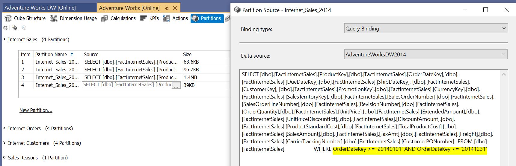
Figure 6a – Partition definition in SSAS.

The considerations for Kyvos partitioning are similar to that of most cloud-based “databases”. That is, a one-two punch of distribution across servers and partitioning of files. For Kyvos, this means aggregations are distributed across a number of Query Engines nodes and those aggregations are partitioned into a number of files.

Figure 6b shows that for Kyvos the “Partition Strategy” is determined by a “base partition” date level attribute, and one or more sub-partition keys.

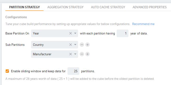
Figure 6b – Partition Strategy for a Kyvos cube

In the end, SSAS MD and Kyvos end up with roughly the same number of files: Partitions X Aggregations. For example, if an SSAS MD cube partitioned a measure group into 5 one-year partitions and each had an aggregation design consisting of 10 aggregations, there would be 50 files.

SSAS MD allows for the aggregations of each partition to reside on different storage devices. However, reading of those partitions is still constrained by the limited number of threads on a single machine. For Kyvos, the partitions of the aggregations reside on a scale-out storage account, sharded across a number of servers.

Aggregation Design

In the physical sense, aggregations are the cube. After all, SSAS MD and Kyvos are mostly about the performance gain from the pre-aggregation of data. In addition to the performance gain from pre-aggregated data, the management of these pre-aggregations is equally relevant to the value of OLAP. So it’s fitting that we end this blog series with Aggregation Design.

Although aggregations are core to SSAS and Kyvos, the aggregation design methods differ considerably. This difference is due to the inherent differences between their respective SMP versus Cloud natures and the attribute-based versus hierarchy-based architecture.

Regarding the SMP vs. Cloud natures, hardware-based performance improvements for SSAS implementations are made primarily through scaling up to a bigger SMP – which has limits. For Kyvos, performance improvements are through scaling out the number of nodes in the Query Engine cluster to as many as is needed to meet response requirements. Of course, it’ll cost you, but it can be done. This expansive scalability is probably the key consideration for migrating from SSAS MD to Kyvos.

Table 3-7 is a map between SSAS MD and Kyvos aggregation concepts.

SSAS Component	Kyvos Counterpart	Description
Aggregation Parameters	Aggregation Strategy	Configurations that affect the automatic creation of an Aggregation Design
Aggregation Design	Call it Aggregation Design for simplicity.	The set of aggregations chosen for materialization
Usage-based Optimization	Smart Aggregates	Features that affect the aggregation design, mostly based on actual user queries.

Table 3-7 – Components of Aggregation

Regarding the attribute-based vs. hierarchy-based nature, we’ll start with a reminder that an aggregation is the sum, count, max, min, etc. of a combination of attributes across various dimensions. For example, an aggregation may hold sales aggregations for the zip code of stores, product category, and month of sale. Or, it may hold the sales aggregations by sales territory, product vendor, and quarter of the sales.

For SSAS MD, a set of such aggregations is called an Aggregation Design. I’ll use the same term for Kyvos. The set can include up to hundreds of aggregations occupying 10s of terabytes of storage, each a unique permutation of attributes/levels from the cube’s multi-dimensional space.

A crucial point to remember is that only a very small percentage of the possible aggregations are included. If that were not true, the act of somehow selecting a set of aggregations wouldn’t be such a big deal. We would just create all aggregations.

That is truer for SSAS MD than for Kyvos. For SSAS MD, the possible aggregations are all the permutations of all attributes of the dimensions. SSAS MD is attribute-based, meaning all attributes could be candidates for aggregations. For even a modest cube, of say 5 dimensions with a total of 30 attributes across those dimensions, the number of permutations with those 30 attributes around 30! (give or take a few trillion) is an astronomical number,

For Kyvos, the possible number of aggregations are the permutations of all hierarchy levels. Only the levels of a Kyvos dimensions hierarchy is eligible for an aggregation. That same cube of 5 dimensions, with say 3 levels each, totals 15 attributes for about 15! (about 1 trillion) possible aggregations. It’s certainly a much smaller number; this still incredibly huge. How long would that take to process, and how much storage would that require?

Fortunately, we don’t need to involve that many permutations. Many permutations will rarely, if ever, be requested. Many high-cardinality aggregations won’t add much value and probably will not be created. And very many queries could be served by a lower-granularity aggregation. For example, an aggregation of stores/year could be served almost as well by stores/month.

SSAS MD’s Aggregation Design Wizard

SSAS’s Aggregation Design Wizard collects various hints from the dimension and cube definitions, member cardinalities, and target metrics (Performance Gain or Storage Size) and searches for a set of aggregates (an aggregation design) that best meets the target metrics. Small aggregates are favored over larger aggregates since they take time to process and store.

The Aggregation Design Wizard outputs a set of aggregations known as the “Aggregation Design”. Determining the set of aggregations is sort of a “Monte Carlo” process. The Aggregation Design Wizard tries and modifies all sorts of combinations until it’s satisfied that there probably isn’t a set that’s much better than the current best set.

When the cube is processed (assume MOLAP), the fact data is copied and aggregated at the lowest granularity. This fact data is the fallback position when there isn’t an aggregation for a query. As a reminder, aggregations are built from this lowest-level “fact data” – the source data is only touched to create the fact data.

Kyvos Aggregation Strategy

Kyvos’ method is more directly methodical. Kyvos instead utilizes a set of parameters under a heading called the “Aggregation Strategy”. The most important settings allow the exclusion of certain hierarchy levels. Kyvos is able to take a more methodical approach because it’s building aggregations off hierarchy levels (where each parent/child level has a 1:m relationship) and not all of the attributes (which are mostly m:m relationships) as SSAS MD does.

Basically, a low-level “root aggregation” is first created. It’s an aggregation at the lowest levels of each dimension hierarchy. It’s actually the same thing as the “fact-level” MOLAP data in SSAS MD. Subsequently, tiers of higher level are derived from that lowest-granularity root aggregation.

Better Aggregations

Both aggregation design methods undoubtedly leave out some needed aggregations and/or create unused ones.

SSAS MD offers a feature called Usage-Based Optimization to help an aggregation design evolve to changing needs. Kyvos’ counterpart to Usage-based Optimization is Smart Aggregations, which make very helpful design recommendations that can be manually or automatically applied. Both analyze query logs for subcubes involved in MDX queries.

SSAS MD has a UI for selecting very specific aggregations that the Aggregation Design Wizard didn’t specify. For Kyvos (and SSAS for that matter), this same result can be obtained by “gaming” the query log used by Smart Aggregations. The idea is to submit the queries requiring the aggregation very many times to “influence” the aggregation design component.

In the end, the aggregations of SSAS MD and Kyvos result in that sub-second query response time for most queries. It’s actually more impressive for Kyvos since those results are based on much more data than typical SSAS MD cubes.

Next Steps

This blog series took a mid-level into the major comparison points between SSAS MD and Kyvos. For anything not covered, or that needs a deep-dive elaboration, please contact us now. We will schedule a meeting with our experts to answer any questions.

Furthermore, these blogs provide more information related to migrating from SSAS MD to Kyvos:

• Migrate Your SSAS Cubes to the Cloud or an On-premise Data Platform
• Kyvos Launches New Utility to Simplify Migration of SSAS Cubes to the Cloud
• Replace SSAS Cubes with Smart OLAP on the Cloud and On-Premise Data Lakes